Benjamin Borketey’s expertise spans fraud detection, data science, data management, prediction, forecasting, Machine Learning, and Artificial Intelligence. With 7 years of experience in the U.S. financial sector, he specializes as a Data Scientist, focusing on developing advanced machine learning models for fraud detection. He has also authored multiple publications on machine learning and has spoken at numerous conferences. He holds a master’s degree in Quantitative Economics and Econometrics from the University of Akron in Ohio. Additionally, he possesses a postgraduate certificate in Machine Learning and Artificial Intelligence from Purdue University.
- Introduction
Financial fraud involves misleading or withholding information from victims regarding promised benefits, commodities, or services frequently to obtain economic advantage. In the U.S. financial sector, identity theft is a common theme in various credit card fraud schemes. Identity theft occurs when a fraudster obtains access to or opens an account using the victim’s personal information, often by stealing utility bills or bank statements. Scams can happen over the phone or through email, with the con artist posing as a bank official and asking for private information. The criminal then reports a missing card to the cardholder’s bank using this personal information, and the bank issues a new card to the criminal.
Credit card fraud occurs through various channels, including online, over the phone (both by text and voice), and in-person. It involves a wide range of illegal activities, such as card skimming, where fraudsters install skimmers on gas pumps, ATMs, and point of sale (POS) systems to steal card information where customers swipe their credit or debit cards. In account takeovers, fraudsters use stolen personal information to contact credit card companies, pretending to be legitimate cardholders.
Credit card application fraud involves using stolen personally identifiable information, such as names, addresses, birthdays, and social security numbers, to apply for credit cards in card-not-present (CNP) and card-present transactions. Other forms of credit card fraud include complex online scams and synthetic identity fraud, where criminals create fake identities using a combination of real and fabricated PII. These fraudulent activities result in significant financial losses and emphasize the need for robust fraud detection and prevention measures.
The growing popularity of credit cards has resulted in a rise in online business transactions and the convenience of electronic payment systems. However, this widespread adoption has also given rise to fraudulent activities. According to the Federal Trade Commission’s Consumer Sentinel Network data book for 2021, the primary types of fraud reported in the United States were identity theft (25.01%), imposter scams (17.16%), issues with Credit Bureaus and online shopping scams (6.94%). Collectively, these fraudulent activities accounted for 50% of all reported fraud cases in the country.
The financial sector is increasingly alarmed by the escalating threat of credit card theft, which results in the loss of billions of dollars to fraudulent activity annually. The impact of credit card fraud is pervasive, affecting not only the individual consumer but also the issuing banks, businesses, and government agencies. The consumer bears the brunt of financial losses and damage to their credit score due to unauthorized charges on their credit cards, impairing their access to loans and other financial services. Larger-scale credit card fraud inflicts a staggering annual revenue loss of billions of dollars on banks. The Federal Trade Commission’s recent data for 2022 revealed that consumers reported a staggering $8.8 billion loss to fraud, a more than 30% increase from the previous year. Furthermore, the FBI’s Internet Crime Report for 2022 highlighted that Credit Card/Check Fraud accounted for $264.1 million in reported losses, while Identity Theft led to $189.2 million in losses.
Fraud detection involves analyzing customers’ transaction behavior to determine the legitimacy of transactions. With the increasing prevalence of electronic transactions, detecting and preventing fraudulent activities has become more challenging. Traditional rule-based approaches adopted by banks and financial institutions often struggle to keep up with evolving fraud techniques and the sophisticated methods employed by fraudsters.
Machine learning has emerged as a powerful and efficient methodology for combating credit card fraud. These systems leverage models trained with historical data on both fraudulent and legitimate activities to autonomously identify characteristic patterns and recognize them when they reoccur. By scrutinizing large volumes of transaction data and pinpointing suspicious patterns, machine learning models can accurately classify transactions as either genuine or fraudulent, providing a robust defense against evolving fraud techniques.
- Research Objectives
This research aims to identify the most efficient methodology for detecting fraud, identify the most important features using the chosen model, and determine the percentage of fraudulent activities detected (detection rate) by the model in the riskiest bin in real-time. Specifically, this research adds value to the current literature by providing a real-time demonstration of an efficient methodology for detecting and preventing fraud and also provides the percentage of fraudulent activities detected by the model in the riskiest bin. Additionally, SHAP values will be employed to study the global and local influence of each feature on fraud. These objectives are crucial in the ongoing battle against credit card fraud, as they will contribute to the development of more effective and robust fraud detection and prevention measures.
- Methodology
The primary research methodology involves comparing various machine learning approaches logistic regression (LR), Linear Discriminant Analysis (LDA), K-nearest Neighbors (KNN), Classification and Regression Tree (CART), Naive Bayes (NB), Support Vector Machine (SVM), Random Forest (RF), XGBoost (XGB), Light Gradient-Boosting Machine (LightGBM) and selecting the best optimal model based on evaluation metrics such as AUC, PRAUC, F1, KS, Recall, and Precision. The chosen model will then be employed in subsequent analyses to determine how features contribute to and explain fraud detection using feature importance scores and SHAP values.
- Data Processing and Feature Selection
The research used a credit card dataset sourced from Kaggle, which consists of transactions conducted by European cardholders over two days in September 2013. The dataset presents transactions that occurred in two days with 492 frauds out of 284,807 transactions. As is customary in fraud datasets, non-fraudulent transactions vastly outnumber fraudulent ones, with 284,315 (99.83%) non-fraudulent transactions and 492 (0.17%) fraudulent transactions. To protect the confidentiality of customer features, Principal Component Analysis (PCA) transformation was applied to the original dataset, excluding identifiable information features such as “time” and “amount.” Thus features V1, V2…V28 are the principal components obtained with PCA. The “Time” feature contains the seconds elapsed between each transaction and the first transaction in the dataset. The “Amount” feature is the transaction amount. The target “Class” is the response variable and it takes the value of 1 in case of fraud and 0 for non-fraud.
To ensure accurate modeling, one of any two features with a correlation coefficient of 0.99 is excluded from the model training process. To address the class imbalance, I used the highly effective synthetic minority oversampling technique. This technique tackles class imbalance in machine learning by generating synthetic samples for the minority class. It identifies the minority class instances, selects their nearest neighbors, and creates new artificial examples along the lines connecting these neighbors, effectively expanding the dataset with realistic representations of the underrepresented class. To address the class imbalance for efficient modeling, the Synthetic Minority Oversampling Technique (SMOTE) is applied to the minority class (non-fraud). This results in a final balanced dataset comprising 199,002 instances of fraud and 199,002 instances of non-fraud.
Figure 1. Top 27 features with the highest importance score.
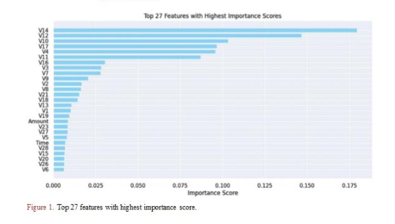 Random Forest feature importance is used to select the top 27 features in the early run. This selection aims to achieve faster training times, prevent overfitting, and improve overall model predictions. Figure 1 shows the top 27 features selected using the Random Forest importance metric. Subsequently, the final dataset, containing only the selected features, is divided into a 70% train set and a 30% test set for further analysis.
3.2. Model Building
The primary research methodology involves comparing machine learning approaches and selecting the best model based on evaluation metrics. An automatic algorithm with 10-fold cross-validation is implemented in the building process to achieve this goal. This process comprises the following models:
Logistic Regression (LR): is a linear classification model that plays a crucial role in binary classification tasks. It predicts the relationship between a dependent variable and one or more independent variables. This model leverages the logistic function, the sigmoid function, to transform a linear combination of independent variables into a probability score.
LR offers interpretability, enabling an easy understanding of the impact of independent variables on outcomes, and allows probability estimation for assessing prediction uncertainty. It demonstrates robustness to noise and irrelevant features, ensuring effectiveness in high-dimensional datasets, and boasts computational efficiency, making it suitable for large-scale applications. However, LR assumes a linear relationship between variables, limiting its expressiveness in capturing complex patterns, and it can be sensitive to outliers, potentially skewing predictions. Additionally, LR is primarily designed for binary classification, requiring modifications for multi-class tasks, and it assumes independence among observations, which might not hold in all scenarios.
Linear Discriminant Analysis (LDA): This model predicts the class of the dependent variable by using the linear combination of the independent variables. LDA aims to maximize class separation while minimizing within-class variance by identifying a linear combination of independent variables. Discriminant functions derived from this process are then used to classify new observations using a designated decision rule. Additionally, LDA can reduce dimensionality by projecting data into a lower-dimensional space while preserving the distinct separation between classes. LDA offers the advantage of dimensionality reduction by projecting data into a lower-dimensional space while preserving distinct class separation. However, LDA can be sensitive to outliers and assumes that independent variables are normally distributed within each class, potentially leading to biased parameter estimates.
K-nearest Neighbors (KNN): KNN, a versatile algorithm, uses proximity to make classifications or predictions about the grouping of an individual data point. It applies to both classification and regression problems, assessing similarity by considering the k-nearest neighbors in the feature space. In classification, KNN assigns a data point to the majority class among its neighbors, while in regression, it calculates the average of their values. This algorithm proves effective for diverse predictive tasks, adapting its approach based on the specific requirements of the problem at hand, giving you a wide range of options to choose from. KNN’s simplicity and adaptability make it accessible to beginners and suitable for diverse predictive tasks. However, KNN’s computational complexity and memory intensity can pose challenges, especially with large datasets, and its predictions may be sensitive to noise and outliers. Additionally, selecting an optimal value for the parameter k is crucial for achieving optimal performance and often requires a great amount of time for experimenting and tuning.
Classification and Regression Tree (CART): CART, a widely used algorithm for predictive modeling and decision-making, can be employed for both classification and regression tasks. It provides a tree-like structure that represents decision rules and splits in the data. In classification, the tree categorizes instances into different classes, while in regression, it predicts numerical values. The interpretability of CART makes it a powerful tool, giving you confidence in your understanding of the model’s decision-making process. CART’s interpretability is a significant advantage, it provides transparency into the model’s decision-making process, which instills confidence in its outcomes. However, CART also has limitations. While it is easy to interpret and visualize, it can be prone to overfitting, particularly when the tree depth is not adequately controlled. Additionally, CART may lack robustness when faced with small variations in the data, potentially leading to unstable predictions.
Naive Bayes (NB): Naive Bayes, a computationally efficient and straightforward algorithm, uses Bayes’ theorem to assign a probability to every possible value in the target class, and the resulting distribution is then condensed into a single prediction. It calculates the likelihood of each class based on observed data and combines it with prior probabilities for making predictions. NB offers quick and effective predictions. Its efficiency provides reassurance about performance, particularly with large datasets. However, NB assumes feature independence, which may not always hold in real-world scenarios. This assumption can limit its ability to capture complex relationships between features, potentially leading to suboptimal performance in certain cases.
Support Vector Machine (SVM): SVM finds a hyperplane that best fits the data points in a continuous space instead of fitting a line to the data points. It can be used in regression and classification tasks. SVM aims to find the hyperplane that maximizes the margin between different classes. While versatile enough for regression and classification tasks, SVM excels particularly in solving classification problems. Its ability to handle complex data and find non-linear decision boundaries makes SVM a powerful tool in various fields of machine learning. SVM’s strengths lie in its effectiveness in high-dimensional spaces and its robustness to overfitting, especially when using appropriate regularization. However, SVM’s computational complexity increases with the size of the dataset, making it less suitable for large-scale applications. Additionally, SVM’s performance heavily depends on the choice of kernel function and its associated parameters and requires careful tuning to achieve optimal results.
Random Forest (RF): Random Forest involves the creation of multiple decision trees, each constructed using distinct random subsets of the data and its features. Each decision tree functions as an individual “expert,” offering its perspective on the data classification. To make predictions, the algorithm computes predictions from each decision tree and ultimately selects the most frequently occurring outcome among these individual results. RF boasts high accuracy due to its ability to reduce overfitting and handle noise effectively. It is versatile, accommodating different types of data, and provides insights into feature importance. However, RF models can be complex and computationally expensive to train, especially with large datasets. Additionally, they may exhibit a bias towards majority classes in imbalanced datasets. Despite these challenges, Random Forest remains widely used and valued for its robustness, accuracy, and versatility in classification tasks.
XGBoost (XGB): XGBoost is particularly popular in various data science and machine learning competitions on platforms like Kaggle due to its high predictive accuracy and versatility. It is designed for classification and regression tasks and is known for its efficiency, scalability, and ability to handle complex structured data. Its success in handling a wide range of datasets and delivering robust performance has made XGBoost a go-to choice for analysts seeking superior predictive models in various applications. XGB advantages include high predictive accuracy, efficient computational performance, scalability to large datasets, and the ability to handle complex structured data. However, XGBoost also has its limitations. It can be computationally expensive, especially when dealing with large datasets and complex models. Additionally, XGBoost’s performance heavily depends on hyperparameter tuning which requires careful optimization to achieve optimal results.
Light Gradient-Boosting Machine (LightGBM): LightGBM is a fast, distributed, high-performance gradient-boosting framework based on decision tree algorithms. It is used for ranking, classification, and many other machine-learning tasks. Its capability to handle large datasets and deliver quick, accurate results makes LightGBM particularly well-suited for applications where speed and performance are crucial, solidifying its popularity in the machine-learning community. However, LightGBM’s performance can be sensitive to hyperparameters, necessitating careful tuning for optimal results. Additionally, its inner workings may pose complexity, demanding a deeper understanding for effective utilization, especially among users less familiar with gradient boosting and decision tree algorithms. While scalability challenges may arise in setting up distributed training environments, there’s a risk of overfitting with high-capacity models.
3.3. Model Selection Metrics
Due to the class imbalance, accuracy may not be the most suitable metric for performance evaluation. Instead, additional metrics, including AUC, F1 score, Precision, and Recall, were employed in evaluating model performance. To ensure a thorough evaluation of the model’s effectiveness in handling class imbalance, PRUAC was incorporated. KS was also included, which quantifies the maximum separation between the cumulative distribution of fraud and non-fraud instances. Descriptions of these performance metrics are provided below.
Accuracy: This metric measures the number of correct predictions made by a model in relation to the total number of predictions made. The range ∈ [0,1].
Precision= : Precision calculates the ratio of correctly classified fraud transactions to all transactions classified as fraud. The range ∈ [0,1].
Recall: This measures the ratio of correctly classified fraud transactions to all actual fraudulent transactions. The range ∈ [0,1].
F1 Score: This combines precision and recall using the harmonic mean. It provides a balanced measure of a model’s performance. The range ∈ [0,1].
Where: TP is the number of transactions correctly classified as fraud.
TN is the number of transactions correctly classified as non-fraud.
FN is the number of fraud transactions wrongly classified as non-fraud.
FP is the number of non-fraud transactions wrongly classified as fraud
KS: The Kolmogorov Smirnov test (KS) measures the maximum separation between fraudulent and non-fraudulent transaction distribution, which is in the range ∈ [0,1].
AUC: This metric summarizes the trade-off between a classifier’s true and false favorable rates. It quantifies a classifier’s ability to distinguish between positive and negative classes—the range ∈ [0,1].
PRAUC: PRAUC summarizes the precision-recall trade-off across different classification thresholds. It calculates the area under the precision-recall curve, which plots precision against recall. A high PRAUC indicates a model that maintains high precision while achieving high recall. This metric is often used for fraud detection, anomaly detection, and imbalanced classification problems—the range ∈ [0,1].
- 4. Results and Discussion
4.1. Model Performance in Train Data
The Random Forest model emerged as the best-performing model, achieving the highest KS score of 99.99% and an AUC of 99.99%, demonstrating its robust ability to effectively distinguish between fraudulent and non-fraudulent transactions in Table 1. The Random Forest model produced the highest accuracy rate of 99.99%, along with the highest precision and recall rates of 99.98% and 99.99%, respectively. This high F1 score of 99.99% signifies a well-balanced trade-off between precise positive predictions (precision) and the comprehensive capture of positive instances (recall) by the RF model. Furthermore, the PRAUC value of 99.99% obtained from the Random Forest model shows its superior ability to differentiate between positive and negative classes compared to all other models. See Table 1.
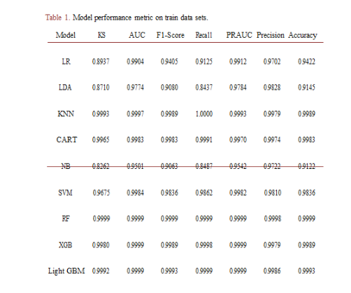 Table 1. Model performance metric on train data sets.
4.2. Detection of Overfitting (Performance on Test Set)
Assessing the performance of the models on the test data is crucial because it provides an unbiased evaluation of how well each model generalizes to unseen data. This evaluation ensures that the models have not merely memorized the training data (a phenomenon known as overfitting) but can accurately predict new, real-world examples. Evaluating performance on a separate, unseen dataset helps determine the model’s reliability and potential to perform well in practical applications, aiding in selecting the best model.
The fitted models are employed to predict the test dataset, and the performance results from the test dataset are compared to those obtained in the training data to detect the possibility of overfitting. Overfitting occurs when a model performs exceptionally well on the training data but fails to generalize effectively to new, unseen data.
Among the models, the Random Forest (RF) model exhibits the lowest reduction in performance metrics when transitioning from the training dataset to the test dataset. A comparison of performance metrics in the training data, as shown in Table 1, to those in the test data, as presented in Table 2, reveals a reduction of less than 20% for all metrics in the test dataset. The RF declined by KS (9.09%), AUC (8.09%), F1-Score (16.47%), Recall (16.15%), PRAUC (16.46%), Precision (16.78%) and Accuracy (0.04%). Consequently, the RF model is selected as the final model for further use in real-time fraud detection and for Shap value explainability.
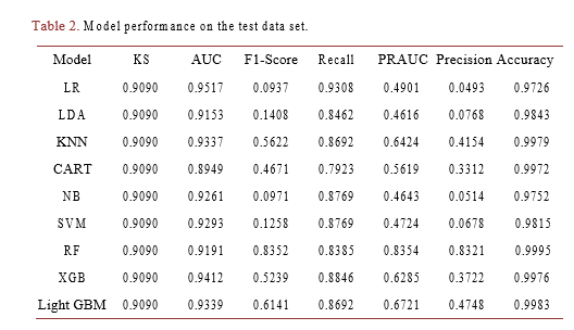 Table 2. Model performance on the test data set.
4.3. Final Model Output and Adjustment
The model output (predicted probabilities) generated by the Random Forest (RF) model were rounded to two decimal points and then multiplied by 100 to bring them within a range of 0 to 100 with one-point increments. In this scale, a score of 100 denotes the highest risk, while a score of 0 indicates the lowest risk.
In real-time fraud detection, the final model output is also converted to a score tie with a set of rules for use in decisions. Based on the score and the rules, a transaction could be approved or sent for manual review pending the customer’s authentication or declined outright. Subsequently, these scores and predicted probabilities were sorted and equally grouped into 10 bins. To assess the appropriateness of this scoring approach, a histogram comparison of predicted probabilities and the score associated with fraudulent transactions in the test dataset was generated.
As depicted in Figure 2, fraudulent transactions exhibit distinct distributions across the binned probabilities and scores. The predicted probabilities and the scores for fraudulent transactions display a right-skewed distribution, with approximately 92% of fraudulent transactions falling within the highest bins, specifically in the ranges [0.9 to 1] and [90 to 100] for predicted probabilities and scores, respectively. Thus, the conversion of the predicted probabilities to scores did not alter the distribution of fraud transactions.
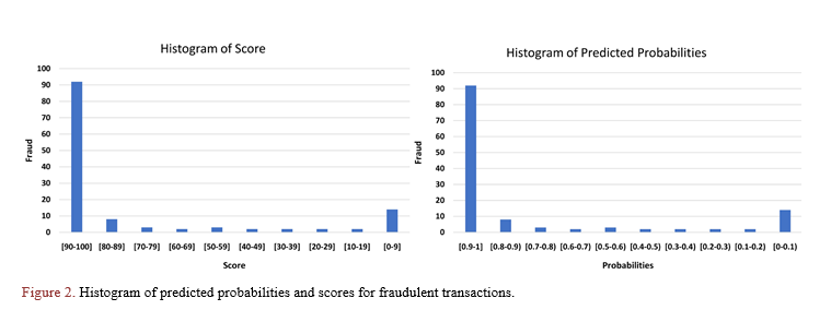 Figure 2. Histogram of predicted probabilities and scores for fraudulent transactions.
4.4. Detection Rate in the Test Data
To assess the detection rate, which represents the proportion of fraudulent transactions detected by the model, a total transaction count per score bin was tabulated, with each bin corresponding to a specific probability range. As illustrated in Table 3, the highest score bin, ranging from 90 to 100, aligns with the highest probability bin [0.9 – 1]. This particular bin contains 92 fraudulent transactions out of 100 transactions. In simpler terms, approximately 92% of transactions scoring 0.9 and above (riskiest bin) are identified as fraudulent, equating to a detection rate of approximately 70.77% at a lower false positive ratio of 0.09 for all fraudulent transactions in the test dataset.
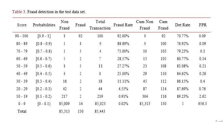 Table 3. Fraud detection in the test data set.
A similar trend is observed across the remaining score bins, where the fraud rate within each bin progressively decreases compared to the riskiest bin in terms of fraud risk. Table 3 also reveals that the RF model captures more than half of the fraud (resulting in a detection rate of over 50%) for each bin in the test dataset. These findings further affirm the Random Forest (RF) model’s robust performance in detecting fraudulent activities in unseen data.
4.5. In Rank Ordering/Monotonicity Testing
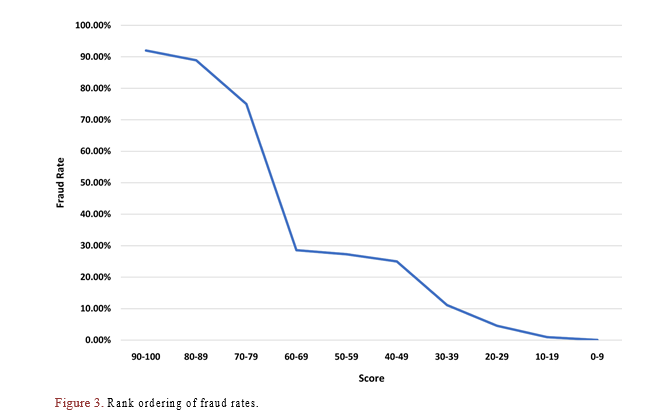
The rank-ordering is a visual assessment that illustrates the model’s ability to consistently rank the fraud rates in decreasing order as the scores decrease. To evaluate this ability, the scores are plotted against the corresponding fraud rates in Table 3. As depicted in Figure 3, the plot exhibits an expected, monotonically decreasing trend in the marginal fraud rate across the score bins. This observation shows the model’s robust rank-ordering ability, exemplified by the highest fraud rate of 92% recorded in the riskiest score bins [90 to 100]. This further reaffirms the best model (RF) model’s ability to detect fraudulent activities.
Conversely, the scores for fraudulent transactions (fraud = 1) display a left-skewed distribution, with a peak in the highest, riskiest score range, as expected. Based solely on visual inspection, the RF model’s discriminatory power is reaffirmed as obtained by the KS and AUC as discussed in Table 1 and Table 2.
- Explainability
Machine learning models are frequently characterized as “black boxes” because of their inherent complexity, which makes it challenging to understand the reasoning behind their predictions. Consequently, there is a growing demand for methods that render these models more explainable and interpretable, shedding light on the intricacies of their predictions. ML explainability is important to ensure algorithmic fairness, identify potential bias in the training data, and ensure that the final model performs as expected.
Machine learning interpretability encompasses a wide array of techniques that are used to clarify and understand the decision-making processes of machine learning models. These techniques include feature importance scores, partial dependence plots, LIME (Local Interpretable Model-Agnostic Explanations), SHAP (Shapley Additive explanations) values, and many others. Among these, SHAP values are often preferred due to their robust theoretical foundation, consistency, and ability to explain complex models by providing coherent feature attributions.
5.1. Shapley Additive Explanations (SHAP)
The use of Shapley Additive explanations (SHAP) for explainability developed by Lundberg and Lee [25] is rooted in cooperative game theory, which distributes the total gain among players according to their respective contributions. Within the game theory framework, the model represents the game’s rules, and the input features are hypothetical individuals who could either play the game (an observed feature) or not (an unobservable characteristic). Therefore, the SHAP technique determines the Shapley values by assessing the model under various feature combinations and figuring out the average difference in the prediction (outcome) between the presence and absence of a feature.
5.2. Global Explainability: SHAP Value Feature Importance Plot
I generated a SHAP summary plot to gain a deeper insight and create a more informative plot to visualize the feature’s importance. This plot organizes the contributions of the features from the most influential to the least influential. Figure 5 summarizes each feature’s impact on the final prediction for the test dataset. The plot clearly shows that “V12” is the most influential feature when making predictions, followed closely by “V14.” Conversely, “V27” is identified as the least important feature, exerting minimal influence on the model’s predictions.
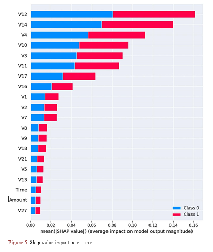 Figure 5. Shap value importance score.
5.3. Local Explainability
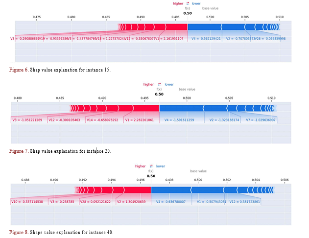
The SHAP values force plot provides local interpretability for each data point predicted by the model. In Figures 6-8, I present force plots generated using SHAP values for the 15th, 20th, and 40th instances, respectively.
These force plots vividly demonstrate how specific features, each with its unique contribution, influence the prediction for each of these instances. Some features exert a positive impact, pushing the prediction higher, while others have a negative effect, pulling it lower. The cumulative effect of all feature contributions adds up to the final prediction value.
In these force plots, features with red coloring indicate contributions that increase the model’s prediction, while features with blue coloring indicate contributions that decrease the prediction. The intensity of the color reflects the magnitude of the contribution. Wider bars on the plot indicate a more extensive range of values for a feature, emphasizing its more significant influence on the prediction.
- Conclusions
The study focused on fraud detection using machine learning; I employed a credit card dataset sourced from Kaggle. After preprocessing and feature selection, I evaluated several machine learning models, including Logistic Regression, Linear Discriminant Analysis, K-nearest Neighbors, Classification and Regression Tree, Naive Bayes, Support Vector Machine, Random Forest, XGBoost, and Light Gradient-Boosting Machine.
The Random Forest model emerged as the top-performing model, showcasing remarkable results in distinguishing between fraudulent and non-fraudulent transactions. It exhibited high accuracy, precision, recall, F1 score, and AUC, demonstrating its robustness in identifying fraudulent activities.
To assess overfitting, I evaluated model performance on a separate test dataset, and the Random Forest model maintained its strong performance, indicating its ability to generalize effectively.
I also explored model interpretability using SHAP (Shapley Additive exPlanations) values. The SHAP summary plot highlighted the importance of individual features, with “V12” being the most influential and “V14” closely following. Additionally, SHAP force plots provided local interpretability, revealing how specific features impacted predictions for individual instances.
In conclusion, the Random Forest model, supported by SHAP values for explainability, represents a powerful tool for real-time fraud detection in credit card transactions. Its strong performance and interpretability make it a valuable asset for financial institutions seeking to enhance security and minimize fraudulent activities.
- Limitation and Future Work
While this study demonstrates the effectiveness of the Random Forest model for real-time credit card fraud detection, there are some limitations to consider. Firstly, although widely used in similar studies, the dataset used in this study is from a European credit card issuer and may not fully represent global fraud patterns. Future research could explore the model’s performance on datasets from different geographical regions to assess its generalizability. Also, as discussed above, PCA transformation was applied to the original data, excluding identifiable information features such as “time” and “amount.” Applying PCA transformation to original data for machine learning introduces challenges such as loss of interpretability and difficulty explaining results due to the transformation of features into orthogonal components. Additionally, PCA may lead to information loss, especially if essential information is discarded. Despite these challenges, PCA remains a valuable technique for dimensionality reduction; future research could explore methods to utilize actual features to mitigate the loss of interpretability.
Secondly, credit card fraud techniques continuously evolve, and fraudsters adapt their strategies to circumvent detection systems. Therefore, the model’s performance may degrade if not regularly updated with new, representative data. Future work could investigate online shopping habits to enable the model to dynamically adapt to emerging fraud patterns.
The RF model is chosen as the best performing model because it requires few hyperparameters to optimize which is advantageous given the limited computational resources. Moreover, the performance of a model could vary depending on the specific characteristics of the data and the problem at hand. The RF model has performed better than other classification models on the European data in the literature. Thus, it would be essential for future research to experiment with another dataset with high computational resources to determine the performance of the model in a different environment or to actual credit card fraud detection system. I would also recommend for future work to consider the real-time and scalability of the model, as well as how it handles the challenges of large-scale data and high-speed transaction traffic.
Lastly, this study focuses on the binary classification of transactions as fraudulent or non-fraudulent. However, fraud detection systems often incorporate additional actions in real-world scenarios, such as manual review or authentication challenges. Future work could extend the model to a multi-class classification problem, incorporating these intermediate actions to better align with real-world fraud management strategies.
- Policy Implication
The findings from this study have significant policy implications for financial institutions, regulators and consumers. The demonstrated effectiveness of machine learning, particularly the Random Forest Model, in detecting credit card fraud in real-time highlights the potential for these techniques to enhance security measures and protect consumers from financial losses.
Financial institutions should consider integrating machine learning-based fraud detection systems into their existing risk management frameworks. By leveraging the power of real-time fraud detection, banks and credit card issuers can proactively identify and prevent fraudulent transactions, reducing financial losses and minimizing the impact on affected customers.
Regulators and policymakers should encourage the adoption of advanced fraud detection technologies, such as machine learning, to strengthen the overall security of financial systems. This could involve providing guidance and incentives for final institutions to invest in these technologies and establishing standards for their implementation and monitoring.
Impact of Borketey’s Works and Overall Contributions to the U.S Financial Sector.
Borketey’s research on Real-Time Fraud Detection Using Machine Learning has many values and significant impacts in the United States and the world at large. See a few outlined below.
Cost Savings and Productivity Boost.
- Adopting Borketey’s models for fraud detection would result in significant cost savings by reducing the need for extensive fraud investigation and legal. Businesses can redirect these savings to other areas potentially boosting productivity and growth. A report by the Association of Certified Fraud Examiners (ACFE) suggests that organizations lose about 5% of their revenues to fraud annually (ACFE Press Release). For U.S. businesses, with a total revenue of approximately USD 30 trillion, this amounts to potential losses of USD 1.5 trillion. If the implementation of Borketey’s models reduces these losses by even 10%, the savings would be substantial amounting to $150 billion annually.
Conflicts of Interest
The author declares no conflicts of interest regarding the publication of this paper.
Copyright © 2024 California Business Journal. All Rights Reserved.


